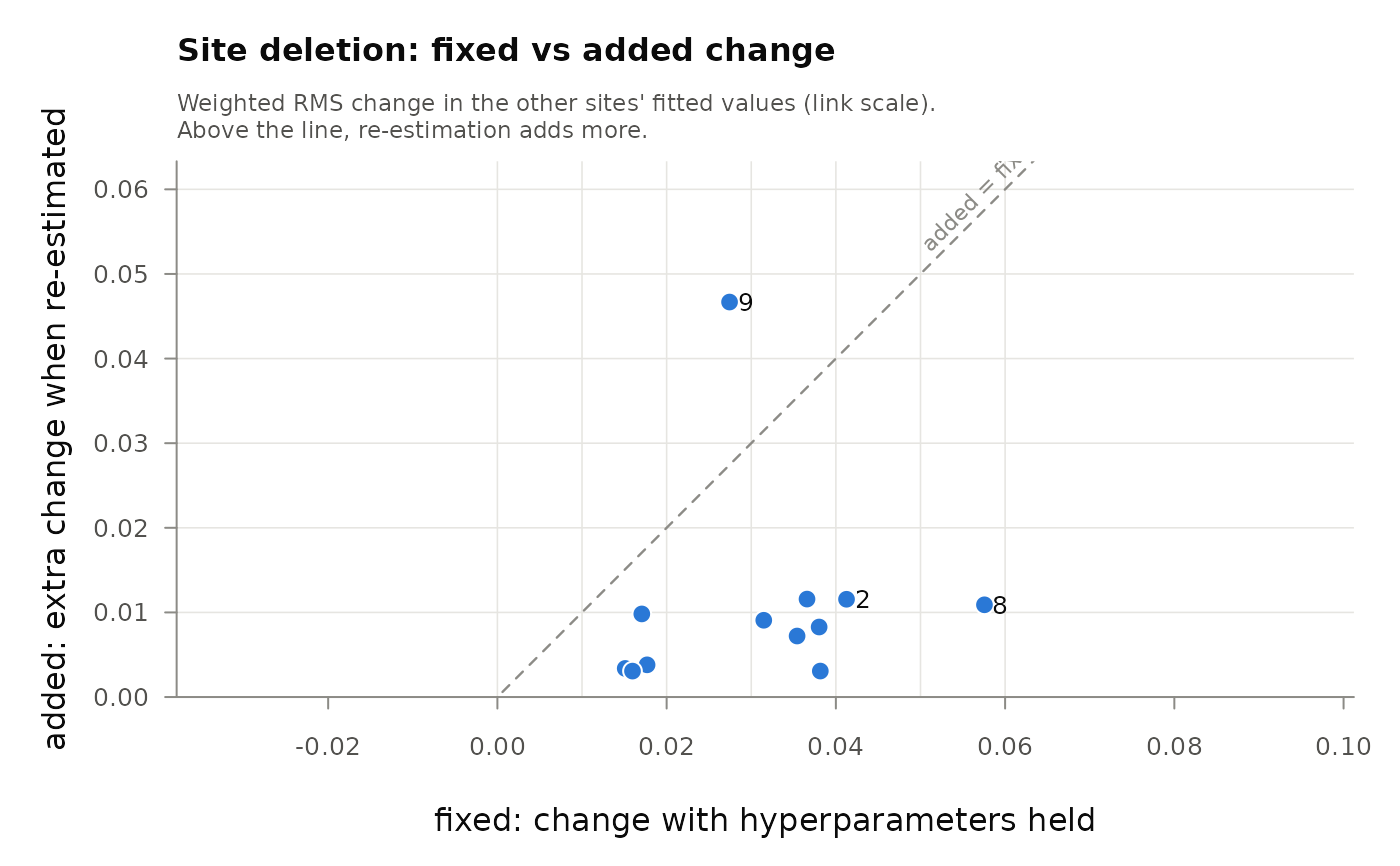
One point per site. The x-axis is fixed, the change in the other sites'
fitted values when the site is removed with the hyperparameters held; the
y-axis is added, the extra change when they are re-estimated. Both are
weighted RMS changes on the link scale (see gam_influence()), so the axes
share one scale. Sites above the dashed diagonal change the fit more through
the smoothing parameters (and theta) than through the held-parameter refit.
Usage
# S3 method for class 'gam_influence'
plot(
  x,
  n = 5,
  by = "total",
  main = "Site deletion: fixed vs added change",
  ...
)Value
Called for its side effect of drawing the plot. Invisibly, a data
frame with one row per plotted site (id, n_obs, fixed, added,
total, status) and a logical column labelled that marks the
labelled sites.
Details
The n sites with the largest by are labelled. Sites whose re-estimated
refit had two REML optima (status "two optima") are drawn as orange
triangles; read their added with care. Sites whose refits failed have no
changes to plot and are left out, with a message.
Examples
library(mgcv)
set.seed(1)
d <- data.frame(site = factor(rep(1:12, each = 6)), x = runif(72))
d$y <- sin(2 * pi * d$x) + rnorm(12, 0, 0.4)[d$site] + rnorm(72, 0, 0.5)
m <- gam(y ~ s(x) + s(site, bs = "re"), data = d, method = "REML")
infl <- gam_influence(m, cluster = "site", progress = FALSE)
plot(infl, n = 3)