Which sites change a GAM, and why? A coral trout example
Source:vignettes/gamfluence.Rmd
gamfluence.RmdThe question
When a model is fitted to data collected at sites, a natural check is
to leave each site out in turn and see how much the fit changes. For a
GAM fitted with mgcv, leaving a site out changes two
things. The coefficients move, and the smoothing parameters, which REML
estimated from all the data, move too. A classical deletion diagnostic
such as Cook’s distance holds the smoothing parameters fixed, so it only
sees the first change.
gam_influence() refits the model twice for every site
and compares the two refits:
- fixed: the site is removed and the estimated smoothing parameters (and a negative binomial θ) are held at their full-data values. This is what a classical diagnostic sees.
- added: what re-estimating them adds on top.
- total: the change when everything is re-estimated.
Each is a weighted RMS change in the other sites’ fitted values, on the link scale. On a log link, an RMS of 0.02 is roughly a 2% change in their predicted means, as long as the individual changes are small.
This vignette runs it on a real model: coral trout on inshore reefs of the Great Barrier Reef.
The data
coral_trout holds 467 surveys of coral trout
(Plectropomus leopardus) at 71 inshore reef sites in the Palm
and Whitsunday island groups, from 2007 to 2018. Each site is fished or
inside a no-take reserve (zoned in 1987 or 2004).
library(mgcv)
library(gamfluence)
str(coral_trout)
#> 'data.frame':    467 obs. of  12 variables:
#>  $ SITE    : Factor w/ 71 levels "B1","B2","B3",..: 1 1 1 1 1 1 1 2 2 2 ...
#>  $ REGION  : Factor w/ 2 levels "Palm","Whitsunday": 2 2 2 2 2 2 2 2 2 2 ...
#>  $ YEAR    : int  2017 2018 2012 2009 2016 2014 2007 2009 2018 2012 ...
#>  $ NTR     : Factor w/ 3 levels "Fished","NTR 1987",..: 2 2 2 2 2 2 2 2 2 2 ...
#>  $ EXPOSURE: Factor w/ 3 levels "Sheltered","Semi-Exposed",..: 1 1 1 1 1 1 1 1 1 1 ...
#>  $ depth   : num  3.94 3.94 3.94 3.94 3.94 3.94 3.94 3.93 3.93 3.93 ...
#>  $ rugosity: num  2.12 2.56 3.24 2.64 3 3.2 3.04 2.16 2.52 2.8 ...
#>  $ LHC     : num  9.6 10.8 34.4 12.4 30 18 25.6 48 42 39.2 ...
#>  $ kd490   : num  0.0751 0.0654 0.0684 0.0668 0.0686 ...
#>  $ maxDHW  : num  6.71 0 1.91 0 3.22 0.6 0 0 0 1.91 ...
#>  $ Cyclone : num  2.391 0.452 1.739 0 0 ...
#>  $ count   : int  18 7 2 19 15 15 15 7 19 3 ...
table(coral_trout$REGION, coral_trout$NTR)   # surveys by region and zone
#>
#>              Fished NTR 1987 NTR 2004
#>   Palm           90       72       18
#>   Whitsunday    140       84       63
The data are derived from Australian Institute of Marine Science (AIMS) data under CC BY 3.0 Australia; the credit is at the end of this vignette.
The model
This is Model A of the coral trout study (Song 2026): a negative binomial GAM with a random intercept for each site, a separate smooth year trend for each region, and smooth terms for habitat and environment.
m <- gam(count ~ REGION * NTR + EXPOSURE + depth +
           s(YEAR, by = REGION, k = 5) +
           s(rugosity, k = 5) + s(LHC, k = 5) + s(kd490, k = 5) +
           s(maxDHW, k = 5) + s(Cyclone, k = 5) + s(SITE, bs = "re"),
         family = nb(), data = coral_trout, method = "REML")
m$family$getTheta(TRUE)       # theta, estimated
#> [1] 5.960065
round(m$sp, 3)                # the eight estimated smoothing parameters
#>       s(YEAR):REGIONPalm s(YEAR):REGIONWhitsunday              s(rugosity)
#>                    0.082                   10.479                    0.868
#>                   s(LHC)                 s(kd490)                s(maxDHW)
#>                    1.120                    0.186                    0.043
#>               s(Cyclone)                  s(SITE)
#>                    0.155                   10.645
Running gam_influence()
One call does the whole analysis. Every site is deleted in turn, and each deletion needs one held refit and one re-estimated refit, so for 71 sites this takes about three minutes:
infl <- gam_influence(m, cluster = "SITE")To keep this vignette quick, it loads the saved result of exactly
that call. The script that made it is
data-raw/coral_trout_influence.R in the package source.
infl <- readRDS(system.file("extdata", "coral_trout_influence.rds",
                            package = "gamfluence"))
A run on two sites takes a few seconds and shows the same numbers:
two <- gam_influence(m, cluster = "SITE", which = c("OE4", "B2"), progress = FALSE)
two$sites[, c("id", "fixed", "added", "total")]
#>    id      fixed      added      total
#> 1  B2 0.01377065 0.01435334 0.02304516
#> 2 OE4 0.02794992 0.06168082 0.07245778
infl$sites[infl$sites$id %in% c("OE4", "B2"), c("id", "fixed", "added", "total")]
#>     id      fixed      added      total
#> 2   B2 0.01377065 0.01435334 0.02304516
#> 43 OE4 0.02794992 0.06168082 0.07245778
Reading the result
Printing the result shows the sites with the largest total change and the largest hyperparameter changes:
infl
#> gamfluence: fixed vs re-estimated deletion, 71 sites
#>   model: Negative Binomial(5.96) (log), 467 rows
#>   status: two optima x18
#>
#> Largest total change in the other sites' fitted values (RMS, link scale):
#>   id n_obs  fixed  added  total
#>  OE4     6 0.0279 0.0617 0.0725
#>  HW2     7 0.0130 0.0651 0.0674
#>   L1     7 0.0146 0.0630 0.0674
#>  OE3     6 0.0186 0.0618 0.0662
#>  OE1     6 0.0099 0.0630 0.0655
#>
#> Largest hyperparameter changes when a site is removed:
#>   id          parameter   full deleted  ratio
#>  HW2 s(YEAR):REGIONPalm 0.0817   11100 135000
#>  OE1 s(YEAR):REGIONPalm 0.0817    8940 109000
#>  PS4 s(YEAR):REGIONPalm 0.0817    7270  89000
#>  OE3 s(YEAR):REGIONPalm 0.0817    6530  80000
#>   L1 s(YEAR):REGIONPalm 0.0817    6480  79300
#>
#> fixed = hyperparameters held; added = what re-estimating them adds.
#> No null reference: compare sites with each other.
The full tables are infl$sites (one row per site) and
infl$hyper (one row per site and hyperparameter).
top_units() sorts the site table by any of the three
changes.
top_units(infl, by = "fixed", n = 5)[, c("id", "fixed", "added", "total", "status")]
#>    id      fixed      added      total     status
#> 1 OS3 0.03890200 0.02158992 0.05344156 two optima
#> 2 OE4 0.02794992 0.06168082 0.07245778 two optima
#> 3 OE2 0.02088804 0.01266547 0.02626593         ok
#> 4 DB2 0.02078453 0.02360840 0.03287249         ok
#> 5  C6 0.02063853 0.01207854 0.02754975         ok
The plot
plot() puts each site at its fixed change (across) and
its added change (up), on the same scale. Sites above the dashed line
change the fit more through the smoothing parameters re-tuning than
through the held-parameter refit.
plot(infl, n = 8)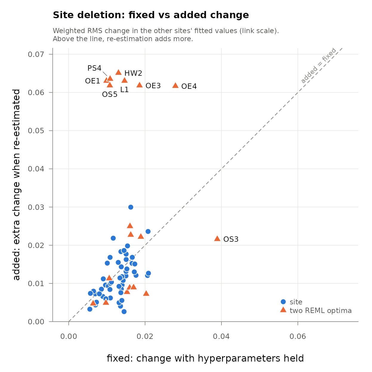
Most sites sit in a cloud near the diagonal. 7 sites sit far above it, at the top left. Held at their full-data smoothing parameters, their deletion looks ordinary: their fixed changes run from 0.01 to 0.028, inside the range of the other sites (0.006 to 0.039). A classical diagnostic would not flag them. Once the smoothing parameters are re-estimated, each of them adds a change of about 0.062 to 0.065, between 2.2 and 6.4 times its fixed change.
Why those sites?
The hyperparameter table shows what moves. For one of them, OE4:
h[h$id == "OE4", c("parameter", "type", "full", "deleted", "ratio")]
#>                    parameter   type        full      deleted        ratio
#> 379       s(YEAR):REGIONPalm lambda  0.08167424 6.246778e+03 7.648407e+04
#> 380 s(YEAR):REGIONWhitsunday lambda 10.47869440 6.522468e+00 6.224505e-01
#> 381              s(rugosity) lambda  0.86790884 2.569041e+00 2.960035e+00
#> 382                   s(LHC) lambda  1.11988867 4.970177e-01 4.438099e-01
#> 383                 s(kd490) lambda  0.18589168 2.922103e-01 1.571939e+00
#> 384                s(maxDHW) lambda  0.04326025 1.765403e-02 4.080890e-01
#> 385               s(Cyclone) lambda  0.15503796 1.160369e-01 7.484418e-01
#> 386                  s(SITE)     sd  0.30650293 3.076471e-01 1.003733e+00
#> 387                    theta  theta  5.96006507 6.067567e+00 1.018037e+00
The smoothing parameter of the Palm year trend jumps from 0.082 to 6,247. A smoothing parameter that large turns a smooth into a straight line: without OE4, the Palm year trend is no longer curved. The same happens for all 7 sites (HW2, L1, OE1, OE3, OE4, OS5, PS4), and straightening the trend moves the fitted values of every Palm site.
Why can one site do that? Fixing the Palm smoothing parameter at a range of values, re-estimating everything else each time, and comparing REML scores shows how flat the score is for that trend:
grid <- c(0.01, 0.1, 1, 10, 1e3, 1e5)
reml <- sapply(grid, function(l) {
  sp <- rep(-1, length(m$sp))
  sp[1] <- l                                  # s(YEAR):REGIONPalm
  as.numeric(gam(formula(m), family = nb(), data = coral_trout,
                 method = "REML", sp = sp)$gcv.ubre)
})
data.frame(lambda = grid, REML_minus_best = round(reml - min(reml), 3))
#>   lambda REML_minus_best
#> 1  1e-02           1.232
#> 2  1e-01           0.000
#> 3  1e+00           0.497
#> 4  1e+01           0.250
#> 5  1e+03           0.087
#> 6  1e+05           0.085
The curved trend (smoothing parameter near 0.1) is the best fit, but a straight trend (very large values) is worse by only 0.085 REML units, with a worse region in between. With two optima that close, removing one site can make the straight line win. For the coral trout study this says the shape of the Palm year trend is only weakly supported by the data, and any conclusion that leans on its curve should be read with that in mind.
Two optima
Because the REML score here has two optima, a single search for the
re-estimated fit can stop at the worse one. gam_influence()
therefore searches twice, from mgcv’s default starting values and from
the full-data values, and keeps the fit with the better REML score. When
the two searches end at clearly different fits, the site’s status says
so and note gives the other fit:
table(s$status)
#>
#>         ok two optima
#>         53         18
x <- s[s$id %in% c("OE4", "W2"), ]
writeLines(paste0(x$id, ": ", x$note))
#> OE4: two REML optima: the better one is used (REML score lower by 0.47); the other gives total 0.0375
#> W2: two REML optima: the better one is used (REML score lower by 0.098); the other gives total 0.0751
For OE4 the straight trend is the better fit after deletion. For W2
the search from mgcv’s defaults stops on the straight-line plateau, but
the curved trend is better, so the curved fit is used. A small REML
difference means the data barely prefer one fit over the other, so treat
those sites’ added and total with care.
Other groupings
cluster can be any grouping of rows, not only sites. For
example, deleting whole surveys (each region in each year):
by_survey <- gam_influence(m, cluster = paste(coral_trout$REGION, coral_trout$YEAR))
plot(by_survey)
How it works
- One representation for every refit. All refits reuse the full fit’s model matrix, identifiability constraints and penalties. So the changes measure the effect of deleting the site, not of rebuilding the basis from less data.
- Two refits per site. The held refit keeps every estimated smoothing parameter (and θ) at its full-data value. The re-estimated refit estimates them again by REML, searched from two starting points.
-
fixed + added = total holds exactly for every
fitted value. The table reports RMS summaries, and those do not add:
totalis never larger thanfixed + added. - A scope guard stops with an error on models outside what the package supports, and a self-check confirms that the refits reproduce the original fit before any site is deleted.
How it is checked
The package’s tests check that the refits reproduce the original fit;
that the held refit matches a closed form and Cook’s distance for a
linear model; that re-estimated refits match ordinary gam()
refits and are optimal under an independently coded REML criterion; and
that row alignment, rank deficiency, two optima and out-of-scope models
are handled.
A known-truth simulation (validation/planted_site.R in
the source) planted one site with an extreme random effect in each of 20
datasets. Its fixed change never exceeded the null 99% line (0 of 20
datasets), while its added change exceeded it in all 20. Its influence
ran through the re-estimated smoothing parameters, which a
held-parameter diagnostic cannot see.
Scope and limits
gam_influence() supports
gam(..., method = "REML") with gaussian, poisson, binomial
and negative binomial families, one-dimensional thin plate smooths,
s(g, bs = "re") random effects and
by = factor; the README lists what is rejected. There is no
null reference or p-value, so compare sites with each other rather than
with a fixed cut-off.
Data credit and references
The coral_trout data are derived from:
Australian Institute of Marine Science (AIMS). (2022). Spatio-temporal dynamics of coral reef fish assemblages on inshore reefs of the Great Barrier Reef. https://apps.aims.gov.au/metadata/view/814a0be3-ed85-4a43-87b7-59ece6eb6a05, accessed 02-Sep-2026. Licensed under CC BY 3.0 Australia.
Based on Australian Institute of Marine Science data.
The model and the study it comes from:
Song, Z. (2026). What explains variation in Plectropomus leopardus density (Version v1.0). Zenodo. https://doi.org/10.5281/zenodo.22933039